One of the most poweful texturing features of POV-Ray is normal
perturbation (which is specified using the normal block
of an object texture). With this feature it's possible to emulate small
surface displacement in a very efficient way, without actually having to
modify the actual surface (which often would increase the complexity of
the object considerably, resulting in much slower renders).
Slope maps are used to define more precisely how the normal perturbation is generated from a specified pattern. Slope maps are a very powerful feature often dismissed by many.
As an example, let's create a simple scene with an object using normal perturbation:
camera { location <0, 10, -7>*1.4 look_at 0 angle 35 }
light_source
{ <100, 80, -30>, 1 area_light z*20, y*20, 12, 12 adaptive 0 }
plane { y, 0 pigment { rgb 1 } }

cylinder
{ 0, y, 4
  pigment { rgb <1, .9, .2> }
  finish { specular 1 }
  normal
  { wood 1
    rotate x*90
  }
}
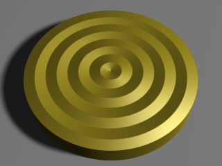
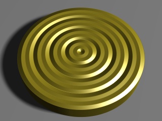
By default the wood pattern uses a ramp wave (going from
0 to 1 and then back to 0) arranged in concentric circles, as we can see
from the image.
By default POV-Ray simply takes the values of the pattern as they are
in order to calculate the normal perturbation of the surface. However,
using a slope_map we can more precisely define how these
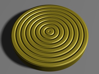
values are interpreted. For example, if we add this slope_map
(the meaning of the values are explained later in this tutorial) to the
normal block in the example above:
    slope_map
    { [0 <0, 0>]
      [.2 <1, 1>]
      [.2 <1, 0>]
      [.8 <1, 0>]
      [.8 <1, -1>]
      [1 <0, 0>]
    }
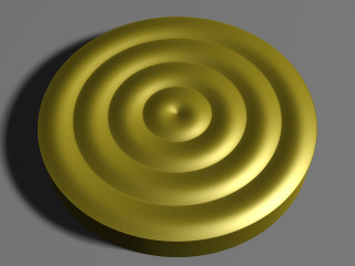
we get a much more interesting result:
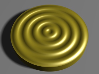
We can also use a slope map to simply smooth out the original ramp wave pattern like this:
    slope_map
    { [0 <0, 0>]
      [.5 <.5, 1>]
      [1 <1, 0>]
    }
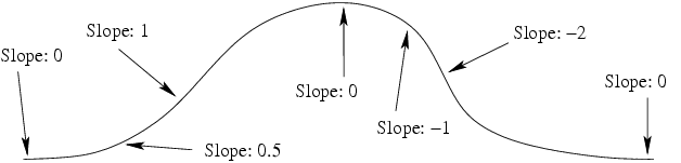
Mathematically speaking the slope of a curve (also called gradient) at
a certain point is the tan() of the angle of the tangent line
of that curve at that point. In other words, it's the amount of change of
the vertical coordinate with respect to the change of the horizontal
coordinate.
In a more colloquial way, the slope of a completely horizontal part of the curve is 0. The slope of a 45-degree line is 1 (because for each unit in the horizontal direction the line goes up by the same amount). Lines between 0 and 45 degrees have corresponding slopes between 0 and 1 (the relation between them is not linear, though, but one usually doesn't have to worry about that). Lines with an angle of over 45 degrees have correspondently slopes increasingly larger than 1 (a line of 90 degrees has an infinite slope).
Usually when defining slope maps it's enough to keep between slopes of 0 and 1, even though higher slopes are sometimes useful too to get steeper changes. Usually it's enough to think that a slope of 0 means a horizontal part of the curve while a slope of 1 means a 45-degree steep part of the curve (and slopes between 0 and 1 correspond to degrees between 0 and 45 respectively).
A slope can be negative too. A negative slope simply means that the curve is going down instead of going up.
The following figure shows some basic slopes in a curve (note that the slope values are only approximate):
In the exact same way as for example a color_map assigns
colors to pattern values, a slope_map assign slopes to
pattern values. If you are fluent in defining color maps for a pattern,
defining a slope map shouldn't be any more difficult.
Each entry in a slope map takes two values: The "displacement" of the surface (although one should remember that this displacement is only simulated, not real) and the slope of the surface at that point.
You can think of the first parameter as an "altitude" value which tells how much the surface (in relative terms) is displaced from its original location. Usually values between 0 and 1 are used for this. You can think of 0 meaning that the surface is not displaced and 1 as the surface having maximum displacement (outwards).
Let's examine the slope map we used to "smooth out" the wood pattern at the beginning of this tutorial:
    slope_map
    { [0 <0, 0>]
      [.5 <.5, 1>]
      [1 <1, 0>]
    }
This means:
When the pattern is linear (as the wood pattern is), this kind of slope map corresponds approximately to a half sine wave. Since the wood pattern uses a ramp wave (ie. after going from 0 to 1 it then goes from 1 to 0), the result is basically a complete (approximate) sine wave.
As with a color map, all the values in between are interpolated and that's why we get a smooth transition between these values.
As we saw in the first slope map example in this tutorial, it is possible to create sharp transitions, not just smooth ones. This is achieved in the same way as how sharp transitions are achieved with color maps: By repeating the same pattern value. Here is an example:
    slope_map
    { [0 <0, 1>]
      [.5 <1, 1>]
      [.5 <1, -.3>]
      [1 <.7, -.3>]
    }
There's a sharp transition at the pattern value 0.5, where the surface goes from slope 1 to slope -0.3 (ie. from going strongly upwards to going slightly downwards). Due to how the wood pattern repeats itself, there are also sharp transitions at the pattern values 0 and 1.
We can combine sharp and smooth transitions for nice effects. For example, this simple slope map achieves a nice result:
    slope_map
    { [0 <0, 1>]
      [1 <1, 0>]
    }
One application where slope maps are really useful is when creating tiled floors. When the tiles on a floor are not too close to the camera and there is a very large amount of tiles, instead of creating hundreds or thousands of individual tile objects, it may be more efficient to simply create a normal pattern which emulates the tiles.
This example shows how to create a floor made of wooden "planks":
camera { location <2, 10, -12>*.5 look_at 0 angle 35 }
light_source
{ <100, 150, 0>, 1 area_light z*40, y*40, 12, 12 adaptive 0 }
sphere { y*.5, .5 pigment { rgb x } finish { specular .5 } }

plane
{ y, 0
  pigment
  { wood color_map { [0 rgb <.9,.7,.3>][1 rgb <.8,.5,.2>] }
    turbulence .5
    scale <1, 1, 20>*.2
  }
  finish { specular 1 }
  normal
  { gradient x 1
    slope_map
    { [0 <0, 1>] // 0 height, strong slope up
      [.05 <1, 0>] // maximum height, horizontal
      [.95 <1, 0>] // maximum height, horizontal
      [1 <0, -1>] // 0 height, strong slope down
    }
  }
}
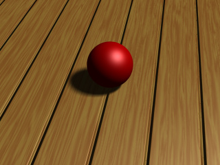
In this case a gradient pattern was used. Since the gradient pattern goes from 0 to 1 and then immediately back to 0, we have to mirror the slope map (around 0.5) in order to get a repetitive symmetric result.
In this example the slope map starts from 0 height and a strong slope up, and goes quickly to maximum height, where the surface is horizontal. Then there's a large horizontal area (from pattern value 0.5 to 0.95) after which the slope goes rapidly back down to 0 height and a strong slope down. (After this there's a sharp transition to the beginning due to the gradient pattern starting over.)
If we want square tiles instead of just "planks", we can achieve that by eg. using an average normal map like this:
  #declare TileNormal =
    normal
    { gradient x 2 // Double the strength because of the averaging
      slope_map
      { [0 <0, 1>] // 0 height, strong slope up
        [.05 <1, 0>] // maximum height, horizontal
        [.95 <1, 0>] // maximum height, horizontal
        [1 <0, -1>] // 0 height, strong slope down
      }
    }
  normal
  { average normal_map
    { [1 TileNormal]
      [1 TileNormal rotate y*90]
    }
  }
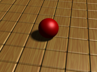
If we change the pigment of the plane a bit, we get a nice tiled floor:
  pigment
  { checker
    pigment { granite color_map { [0 rgb 1][1 rgb .9] } }
    pigment { granite color_map { [0 rgb .9][1 rgb .7] } }
  }
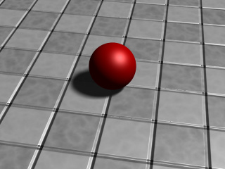
As you can see in the image, close to the camera it's more evident that the tiles are not truely three-dimensional (and that only a normal perturbation trick has been used), but farther away from the camera the effect is pretty convincing.